Figure 1 : are commands lines really that evil :)
Students do not like the command line i.e. command prompts, terminals etc. Some staff members have argued that we should delete Windows and only use Linux in an attempt to wean students off their "point and click" addictions :). However, i decided to try a halfway house, write some software for the students that would generate the required command line strings i.e. a GUI front end, a launcher for the command line assemblers (Link) and simulators (Link) (Link) used in the SYS1 module. A key point to note here is that these GUIs do not replace the command line tools, command line is good, they just generate the correct commands needed to call these programs. The aim is to ease students into using the command line, not to replace it with another "point and click" alternative i.e. the GUI does not support all the command line options, just enough to get you started :). I should add this page also contains the minimalCPU software as well, all one big happy family :).
NOTE: i will not be updating the software in the above links any more, rather the latest versions of any of the simpleCPU software will be available on this web page i.e. you will now only have to download one zip using this link:(Link).
MinimalCPU Instruction Set Simulator Software v2.0
SimpleCPU Assembler Software v2.0
SimpleCPU Instruction Set Simulator Software v2.0
SimpleCPU Instruction Set Simulator Software v2.1
SimpleCPU Instruction Set Simulator Software v2.2
SimpleCPU Assembler and Instruction Set Simulator Software v3
Animated MinimalCPU Instruction Set Simulator Software v1
Before looking at the new GUI I am first going to give a really quick introduction to this processor's command line simulator and its assembly language. For a more detailed discussion of this processor's very unique architecture i.e. its a conceptional machines, rather than a machine that could be implemented in hardware, please refer here: (Link). Note, well it could be implemented in hardware, but that was not its purpose :)
The command line simulator for this processor can be passed the parameters shown below in figure 1.
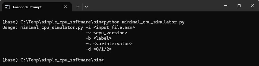
Figure 1 : minimalCPU simulator command line parameters
There are three versions of this processor each expanding on the previous, adding new instructions to its instruction-set. Later versions are backwards compatible to older versions. In the simulator the processor version is specified by the "-v" parameter, default is version 1.
The purpose of this processor is to introduce students to assembly languages, boil things down to basic concepts. So, with that in mind i removed the concept of "memory" i.e. traditional RAM and ROM. Now we just have instructions, labels and variables. Variables are identified using the letters A - Z, so that we can ignore the concepts of addresses and data. To assign a variable a value before run-time we can use the "-s" parameter e.g. -s a:5 assigns 5 to variable a. The default value of each variable is 0.
A program is just a list of instructions, lines of text in a file. Instructions can be identified by their line number, starting with instruction 0, line 0, the line number is incremented by 1 each time a new instruction is added to the text file. An example program (test_minimal_v1.asm) is shown below (Link):
###################
# INSTRUCTION-SET #
###################

#############
# VERSION 1 #
#############

# ADD X Y       ADD X 0
# AND X Y       AND X 0
# JPZ

start:
  AND A 0       # a = 0
  ADD A 2       # a = 2

test1:
  AND B 0       # b = 0
  ADD B 4       # b = 4

test2:
test3:
  ADD A B       # a = 2 + 4 = 6
  AND A B       # a = 6 & 4 = 4

  JPZ start     # jump not taken as a != 0

  AND X 0       # x = 0

  JPZ start     # jump is taken as x == 0
To identify lines / instructions in a program an instruction can be given a label e.g. in this example the instruction AND A 0 is given the label start. Labels identify one instruction, and are names ending with a ":". Note, comments are identified by a '#', you can not have comments on lines containing labels. You can have as many labels as you desire, you can also assign an instruction multiple labels e.g. in the above example test2 and test3, both are assigned to instruction ADD A B, but one could argue why this feature is needed :). Labels are used by the JPZ instruction to identify its branch target i.e. where the program will jump to, if the jump is taken. Labels are also used in the simulator to set breakpoints i.e. when the simulation reaches an instruction with a corresponding label the program simulation is halted, paused to allow the user to examine variables etc. To assign a breakpoints we use the "-b" parameter e.g. -b test1.
The "-d" parameter allows the user to define the debug level i.e. set the amount of "helpful" text printed to the screen as the simulator runs. Default is 0, which is off. The final command line parameter is the "-i" parameter which defines the assembly language file that the user wishes to simulate. Note, the simulator simulates the raw ASCII text, the raw Assembly language, it does not assemble this code i.e. convert it into machine code. An example command line command is shown below:
python minimal_cpu_simulator.py -s a:1 -s b:2 -s c:3 -d 2 -v 3 -b test1 -i test_minimal_v2.asm
In previous labs students would type out these types of command. However, command prompts can be confusing to some students e.g. drive letters C:, D:, H:, then we have the commands: move, copy, cd, dir etc. It surprising how much command line knowledge / teaching has be removed from A-levels. When students get to University very few have used a command prompt, or terminal. Therefore, to ease people into using the minimalCPU command line simulator we now have the GUI shown in figure 2. As always written in python using tkinter.
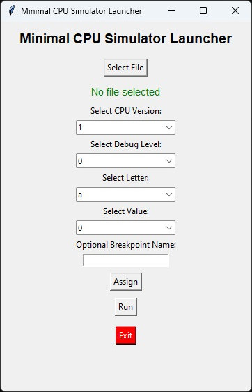
Figure 2 : minimalCPU GUI
On the lab PCs the python environment is setup using Anaconda (Link), i guess for convenience when using Windows. Instructions on how to install this software in Windows at home can be found here: (Link). However, any python environment will do i.e. if you can run these commands all is good. In Linux python is installed by default and these GUIs has been written to work on both operating systems using python3.
Download the code.zip achieve of your choice (version-1), (version-2) or (version-3) and unzip somewhere, i would select version-3 (latest bug fix) and unzipped it to C:\temp, as shown in figure 3s below:
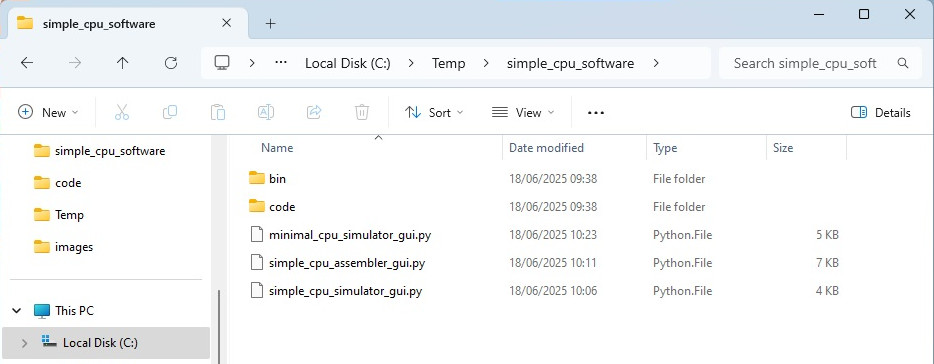
Figure 3a : simpleCPU software folder structure, top-level: gui code
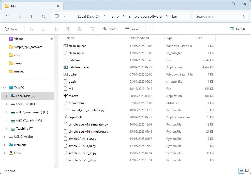
Figure 3b : simpleCPU software folder structure, bin: application code
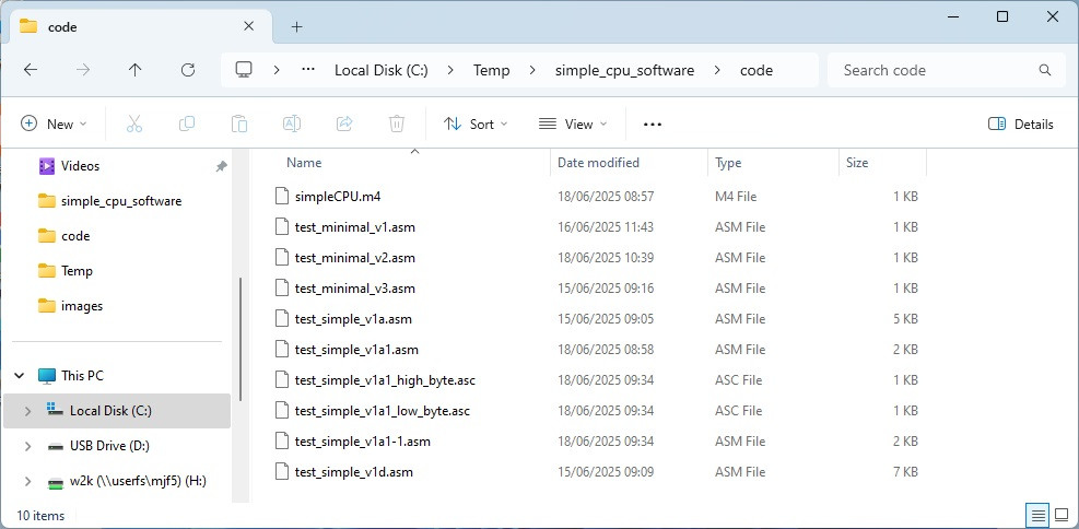
Figure 3c : simpleCPU software folder structure, code: source code
Within the top-level simple_cpu_software folder there are the three GUI applications and a couple of sub-directories (folders). To keep things tidy all the command line tools i.e. assemblers and simulators, are located in the bin directory. Source code i.e. assembly code, is stored in the code directory. This avoids clutter in the top-level directory, only the final output files are copied into this directory, all intermediate object files are stored in the code directory. To help get things started the programs provided in the code directory are basic test code examples, use to test the assembler and simulators. Note, you can store your assembler code in any directory, it does not need to be stored in the code sub-directory.
The three GUI applications are:
In Windows to start this GUI open an Anaconda prompt, shown in figure 4, in Linux open terminal i.e. CTRL + ALT + T.

Figure 4 : Anaconda prompt icon
Next you need to change directory to where you unzipped the simple_cpu_software.zip file i.e. move into the simple_cpu_software folder. To do this on the Windows machines in the lab, first identify what drive (disk) you are using. On the lab machines we have four disks:
In Windows the drive letter is displayed at the start of the Anaconda prompt e.g. in figure 5 we are on the H: drive. I unzipped my code to C:\Temp, therefore, i need to switch to the C: drive. To do this simply type "C:" at the prompt and press the RETURN key. If you are using Linux you don't need to worry about all of this drive letter stuff :).
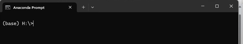
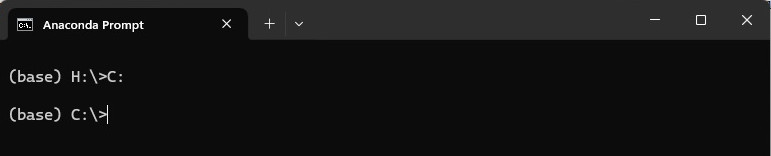
Figure 5 : Anaconda prompt moving from H: to C:
The to move into the simple_cpu_software folder you can use the change directory command: cd:
cd c:\Temp\simple_cpu_software
To check that you are in the correct directory your can use the directory listing command: dir as shown in figure 6. Note, you can also check that you are in the correct directory by examining the command prompt. In Linux you have the same cd command, but none of that drive letter confusion, all storage is mounted from a common route directory i.e. "/". In Linux you would typically unzip the simple_cpu_software.zip file into your home directory, so for me that would be /home/mike. To view the contents of a directory we have a different directory list command: ls. Confess skipping over the Linux usage a little, as in general people using Linux know how to use a terminal :).
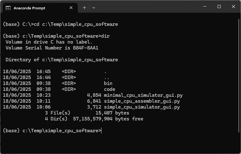
Figure 6 : CD and DIR commands.
To start the GUI, at the command line enter the appropriate command below and press the RETURN key.
WINDOWS : python minimal_cpu_simulator_gui.python
LINUX   : python3 minimal_cpu_simulator_gui.python
This will start the minimalCPU GUI and within the command prompt the program will display the command line command that was used to start it.
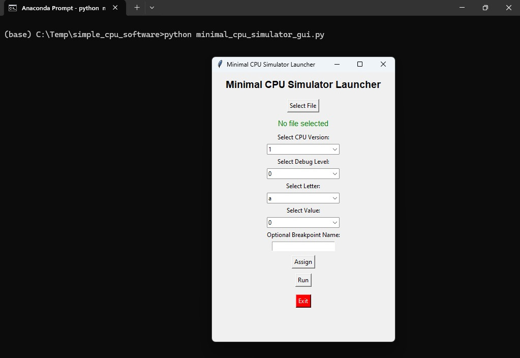
Figure 7 : minimalCPU GUI and Anaconda prompt
Click on the Select File button, this will open a new window allowing you to select the asm file that you wish to simulate, as shown in figure 8. Select a file and then click on the Open button to return to the GUI. Note, for the minimalCPU there is no need to assemble the code first, example code is available in the code directory.
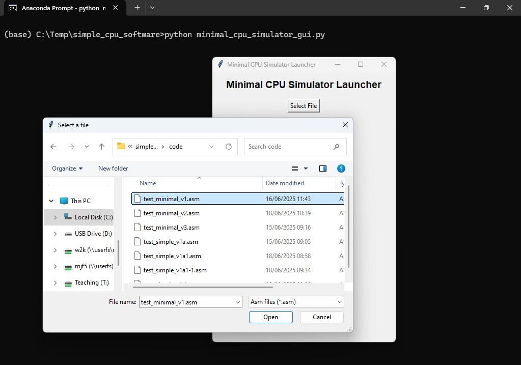
Figure 8 : minimalCPU simulator command line parameters
The green text under this button will be updated to the name of the file selected. Next using the pulldown menus select the CPU version and Debug level needed. To assign a value to a variable click on the letter pulldown menu, select a letter (variable), then click on the value pulldown menu and select a number from 0 to 255 i.e. an 8bit value. To make this assignment click on the Assign button, a green text message will be displayed at the bottom of the GUI confirming that this value has been assigned to the variable. Assignments can be made to multiple variables, repeat this process as needed.
The textbox "Optional Breakpoint Name" allows the user to enter a breakpoint i.e. a label name, at which the user wishes the program to be halted. To simplify the GUI only one breakpoint can be declared. If the command line is used, multiple breakpoints can be declared using multiple -b parameters. Finally, to launch the command line simulator from the GUI click on the Run button. This will open a new command prompt / terminal window allowing the user to step through / run the selected program, as shown in figure 9.
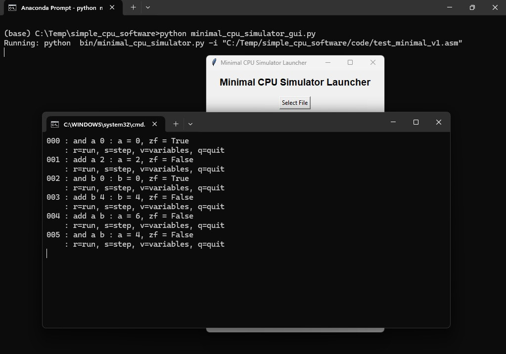
Figure 9 : minimalCPU simulation
To operate this simulator use the following keys:
Note, the command used to launch this simulator is printed to the screen i.e. at the top of the screen in figure 9, showing the user what command they would need to type if they were to run this command manually.
The minimalCPU simulator: minimal_cpu_simulator.py is located in the bin folder. To run these commands manually you can cd into the bin directory, but like the GUI based programs it is recommended to run these from the top level directory. Therefore, cd into the simple_cpu_software top-level directory, then enter the appropriate command below and press the RETURN key.
WINDOWS : python bin\minimal_cpu_simulator.python -v 1 -i code\test_minimal_v1.asm
LINUX   : python3 bin/minimal_cpu_simulator.py -v 1 -i code/test_minimal_v1.asm
This will again launch the minimalCPU simulator, instructions can be executed one at a time by pressing the "s" key, or automatically by pressing the "r" key. Note, the file test_minimal_v1.asm is a test program for the minimalCPU, version 1, stored in the code sub-directory. Breakpoints can be added to the command line to pause the execution of the program at key points. To illustrate this enter the appropriate command below and press the RETURN key.
WINDOWS : python bin\minimal_cpu_simulator.python -b test1 -b test2 -i code\test_minimal_v1.asm
LINUX   : python3 bin/minimal_cpu_simulator.py -b test1 -b test2 -i code/test_minimal_v1.asm
Press the "r" key to automatically step through the program, the simulator will execute an instruction every 0.25 seconds until it reaches the test1 label. At that point the simulator will halt and display the key options, allowing the user to view the state of the last instruction executed, or the state of the processor's variables etc. The user can then press the "r" key to continue the programs execution, or the "q" key to quit. Pressing the "q" key will trigger the simulator to print the value of each variable before stopping the simulator, as shown in figure 10.
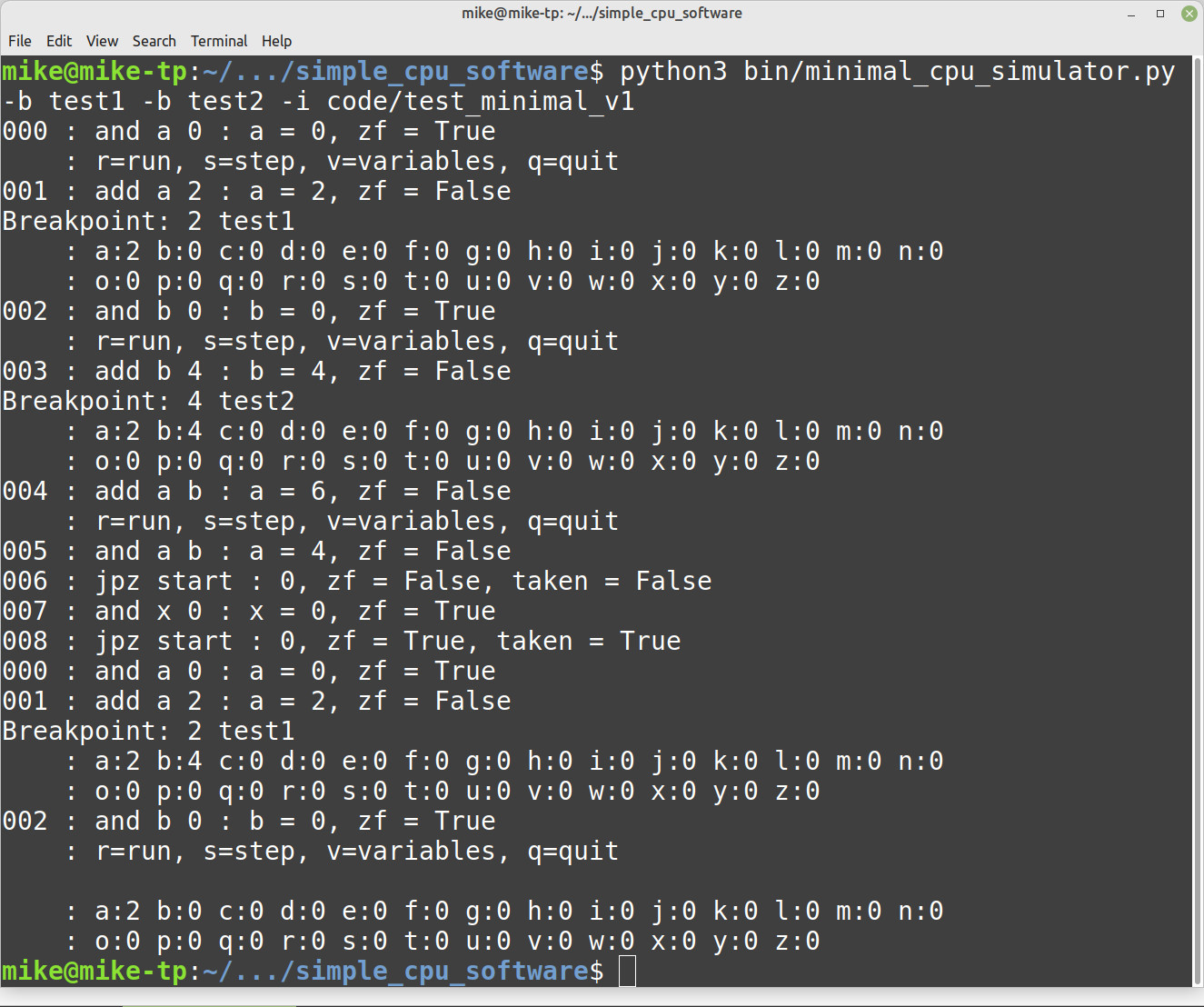
Figure 10 : minimalCPU simulation trace (Linux)
Unlike the minimalCPU simulator i decided to implement a machine code simulator for the simpleCPU i.e. rather than an ISS that simulated assembly language. The reason for not simulating the assembly language program directly was to allow the simulator to support self modifying code i.e. a programming technique that allows a program to rewrite itself at run time (Link). Therefore, before you can simulate a simpleCPU assembly language program you must first assemble it i.e. generate its machine code, a .dat file.
To start the simpleCPU assembler show in figure 11, enter the appropriate command below and press the RETURN key.
WINDOWS : python simple_cpu_assembler_gui.py
LINUX   : python3 simple_cpu_assembler_gui.py
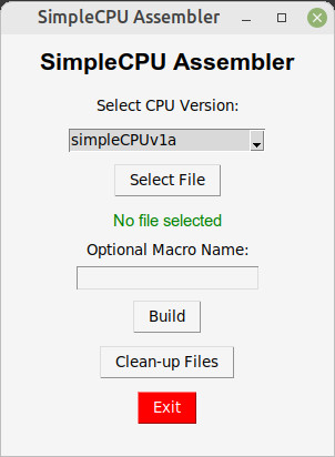
Figure 11 : simpleCPU assembler.
Click on the Select CPU Version pulldown menu and select either version 1a or 1d. These are the only two versions supported at the moment. Next, click on the Select File button, this will open a new window allowing the user to select the asm file that they wish to assemble. Select a file and then click on the Open button to return to the GUI. Note, example code is available in the code directory for testing purposes.
The green text under the button will be updated to the name of the file selected. The textbox "Optional Macro Name" allows the user to enter a m4 pre-processor macro file. More information on macros is available here: (Link). To assemble the assembly language program press the Build button. This will display the required command line command in the command prompt (terminal) and run the selected assembler from the bin directory. Any syntax errors will be displayed in the command prompt. To test this assembler, assemble the file test_simple_v1a.asm, located in the code directory, as shown in figure 12.
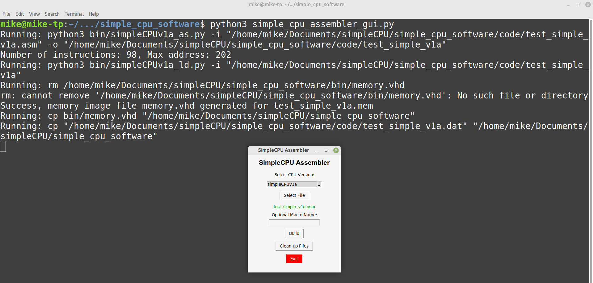
Figure 12 : simpleCPU assembler in action (Linux).
The required command-line command is printed on the screen. The different output files / object files produced by the assembler are stored in the code directory. For ease of use the following files are automatically copied to the top level directory i.e. the simple_cpu_software folder:
To remove temporary files or object files in the code directory and the top-level directory press the Clean-up Files button, again the required command line commands are printed to the screen, as shown in figure 13. The final button, is the Exit button that will close this GUI. This program also automatically creates the file: archive.zip. Each time the Build button is pressed this zip files is updated with a time stamped folder containing backup copies of the above files and their source files, just in case you accidentally delete something, as shown in figure 14.
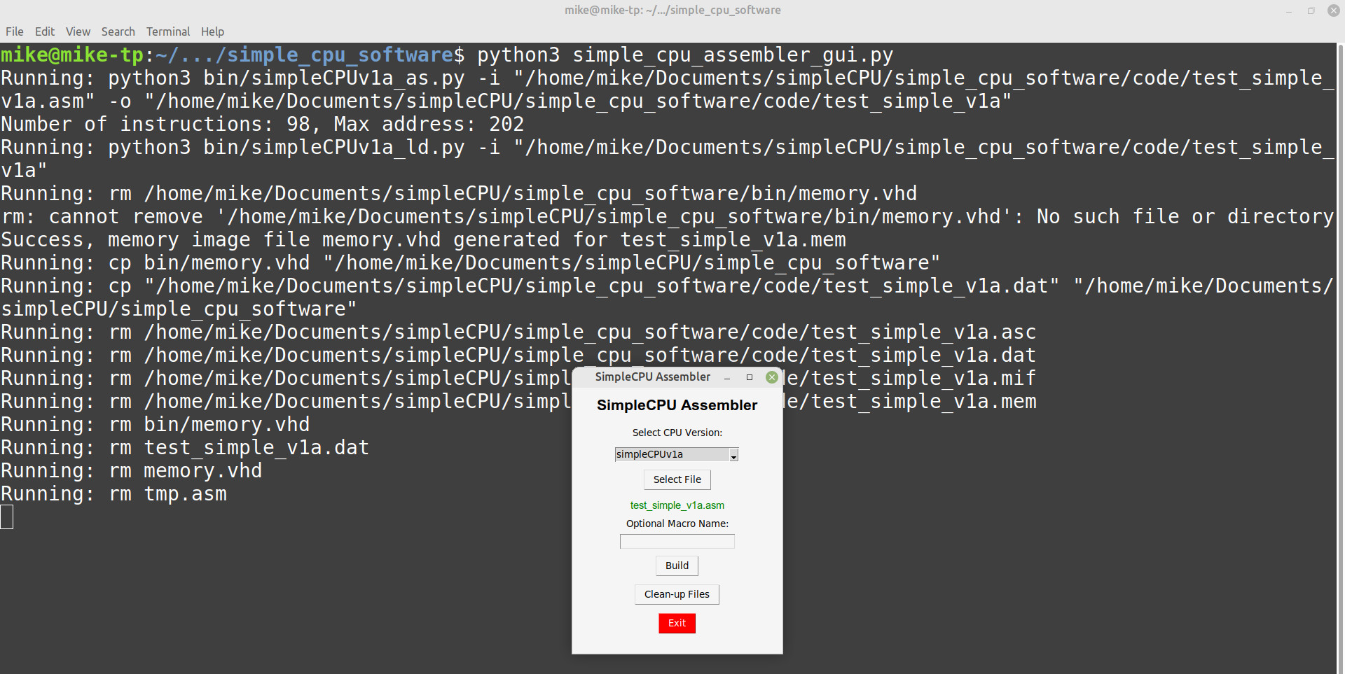
Figure 13 : clean-up (Linux)
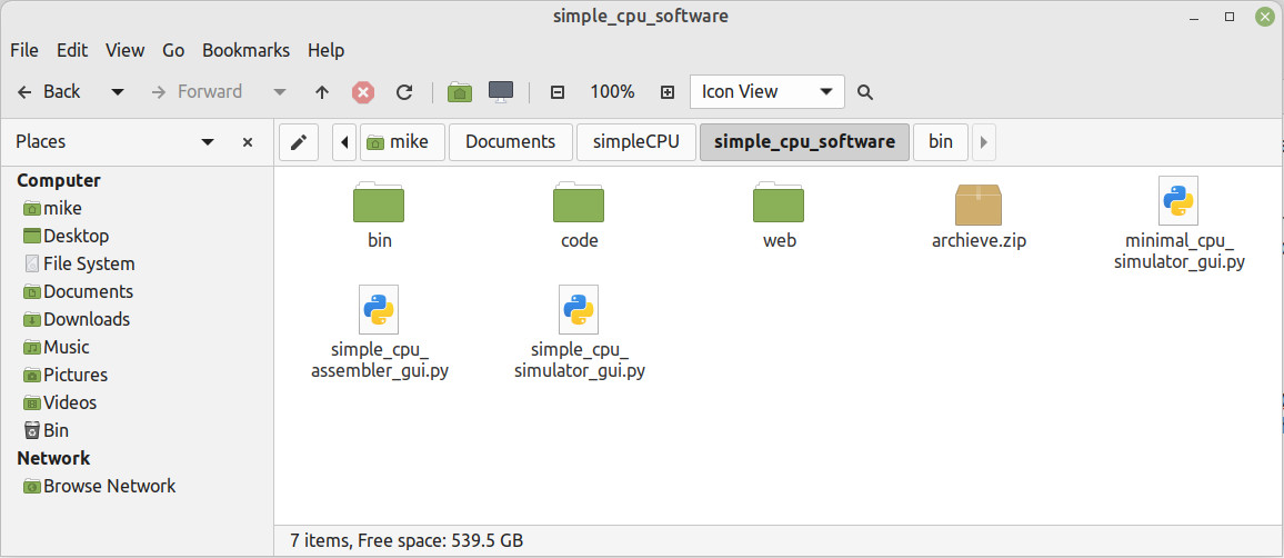
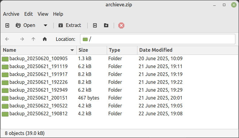
Figure 14 : achieve.zip and zip file structure
The input file used by this instruction set simulator (ISS) is the .dat file produced by the SimpleCPU assembler i.e. you can not directly simulate .asm files. The simpleCPU command line ISS GUI is shown in figure 15. As always written in python using tkinter. Apart from the different input files, the operation of this ISS is basically the same as the minimalCPU.
To start the simpleCPU simulator, enter the appropriate command below and press the RETURN key.
WINDOWS : python simple_cpu_simulator_gui.py
LINUX   : python3 simple_cpu_simulator_gui.py
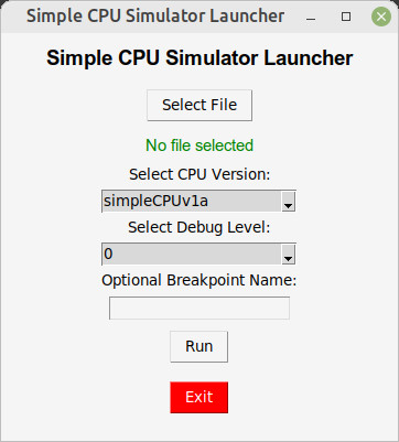
Figure 15 : simpleCPU GUI
To operate this simulator use the following keys:
The v key displays register values, rather than "variables". The user may also view the data stored in any memory location by pressing the m key and entering its address. Finally, when the user exits the simulation by pressing the q key the value of each non-zero memory location is printed to the screen as shown in figure 16.
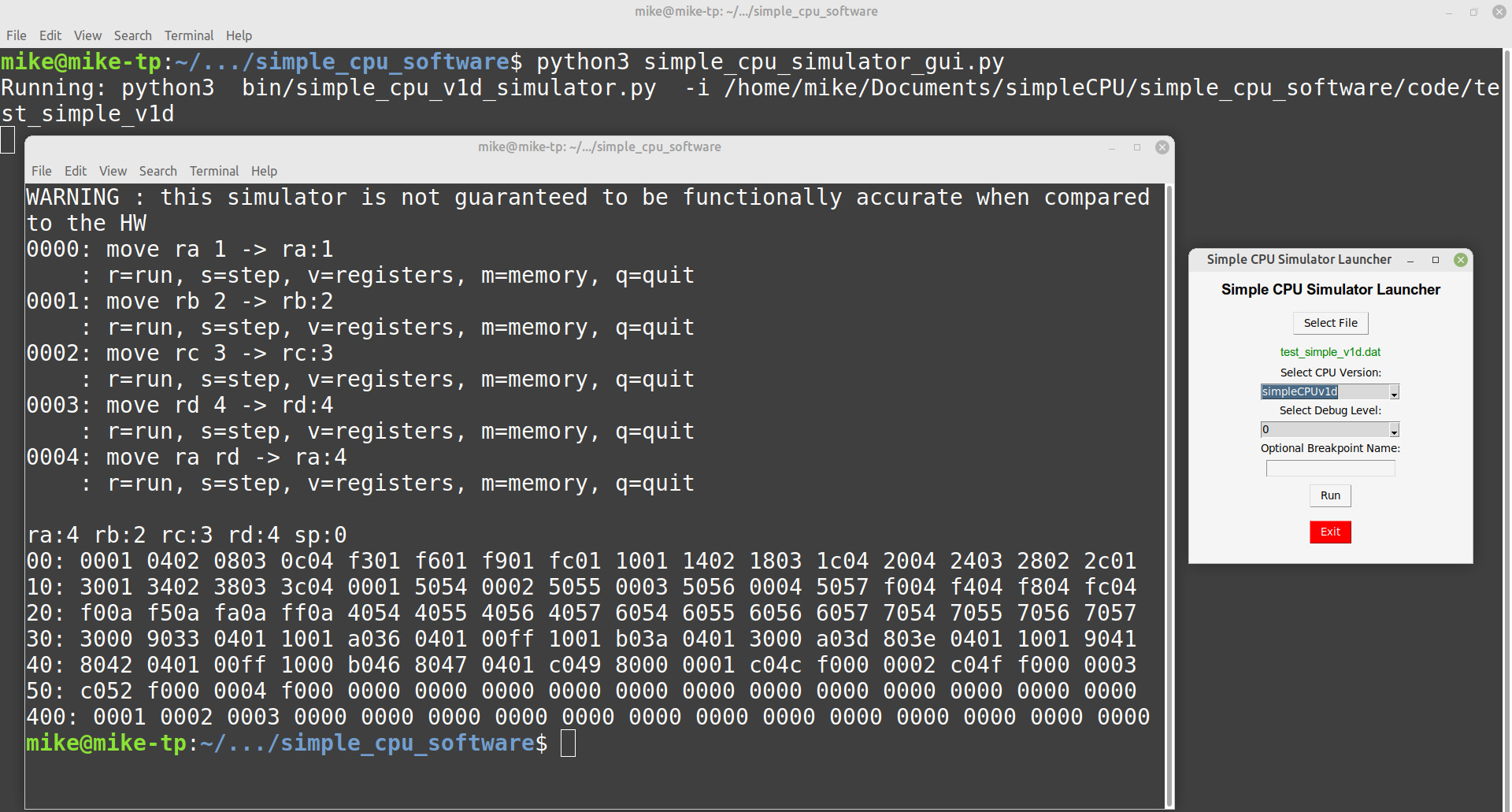
Figure 16 : simpleCPU sumulation trace (Linux)
Another day another improvement :). I've been thinking about how these simulators can be integrated into lab work. In the first simpleCPUv1a lab we look at how memory mapped GPIO is used to interface the simpleCPU to the real world. Implemented on an FPGA this system has two GPIO ports: PORTA and PORTB. These are 8bit interface devices, each having an 8bit input port and an 8bit output port. These are memory mapped devices, therefore, from the processor's point of view they are just “memory” devices. GPIO data can be accessed using the LOAD and STORE instructions i.e. by reading / writing, from / to their assigned addresses, as shown in figure 17.

Figure 17 : memory map, read (left), write (right)
Attached to these IO lines are sensors and actuators, i.e. a bug trap (Link), a piece of hardware that can be controlled by the simpleCPU. Its inputs and outputs are shown in figure 18. Note, port B is not used in this example.
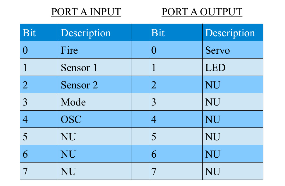
Figure 18 : input and output pins
A key point to note is that access to each GPIO port is dependant not just on the address used, but also the memory transaction type i.e. is the CPU performing a read or a write operation. This added "complexity" was a design decision taken to replicate the behaviour commonly found in peripheral devices seen in the real world. An example from my past, the 68332 micro-controller (Link), so much pain, sleepless nights :). On this micro-controller a number of its onchip peripheral devices used this behaviour e.g. the SCDR - SCI Data Register shown in figure 19.
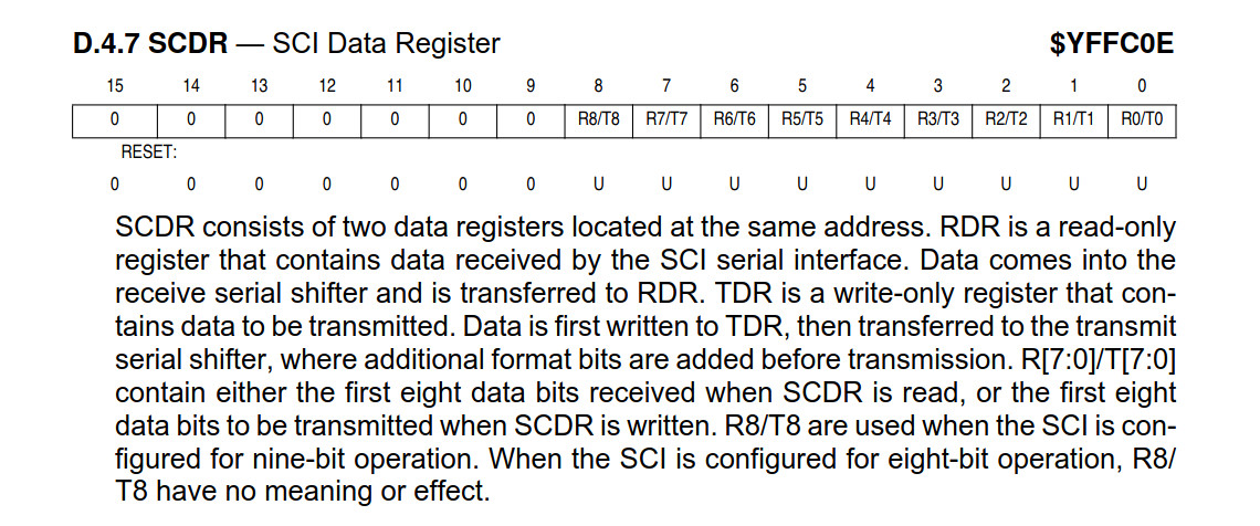
Figure 19 : SCDR - SCI Data Register
Read and writing to the same address triggers different functionality e.g. reading a memory location will also clear processor flags etc. Supporting this behaviour in the simulator helps students to differentiate these types of peripheral devices from memory. In the lab when you write a value to address 0xFC the data is stored to output port-A. When you read address 0xFC you do not read the value of the output port, but rather the data from input port-A i.e. you would not read back the value you wrote. This behaviour is defined graphically using a memory-map, as shown in figure 17. If address 0xFC was mapped to a normal RAM cell you would see a different behaviour, you would simply read back the previously written value. Note, when using micro-controllers / peripheral devices you MUST always read the data-sheet first :).
I confess, rather than coming up with a general solution to incorporating GPIO into the simulator, i have hard coded it to save time. In the future i would like the simulator to have two memory spaces IO and RAM, what is mapped into these spaces would be defined using a text file like that shown below:
ADDR   R/W    TYPE      SIZE
0xF0   W      OUTPUT    8
0xF1   R      INPUT     4
0xF2   RW     RAM       16
Just a thought, however, for the moment gone for a simple solution that fulfils the labs requirements. To enable this GPIO functionality there are a few more command line options, as shown in figure 20. Note, these are not integrated into the GUI at the moment.
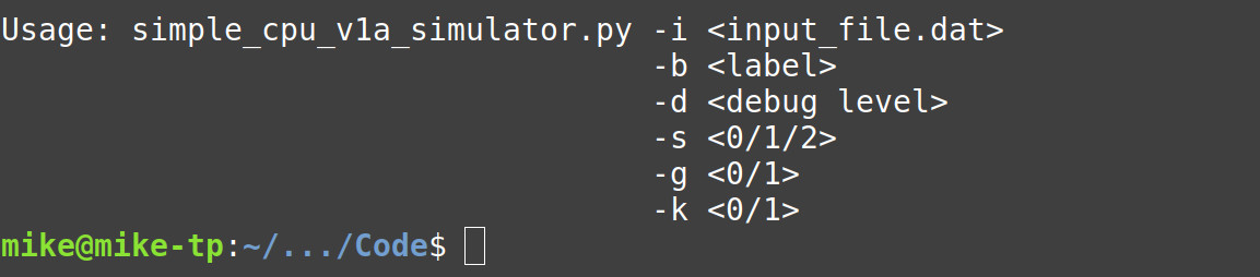
Figure 20 : command line switches
As the GPIO functionality is not needed all the time the user can turn this on or off using the -g parameter, 0=RAM, 1=GPIO+RAM. The -s parameter is speed, by default when the user presses the r key during a simulation the simulator will execute an instruction every 0.25 seconds. This speed was selected so that the user could keep track of what instructions have been executed. Now the user can select different speeds: 0=0.25s, 1=0.05s 2=0s. Default is 0.25s. Finally the -k parameter turns off the key prompt message, 0=off, 1=on. Default is key prompts on. When stepping through a program i found it easier to read the instructions and the updates to registers with this message turned off, examples shown in figure 21.
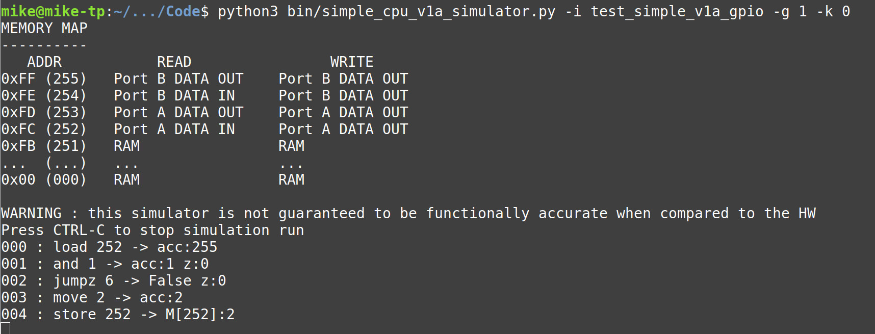
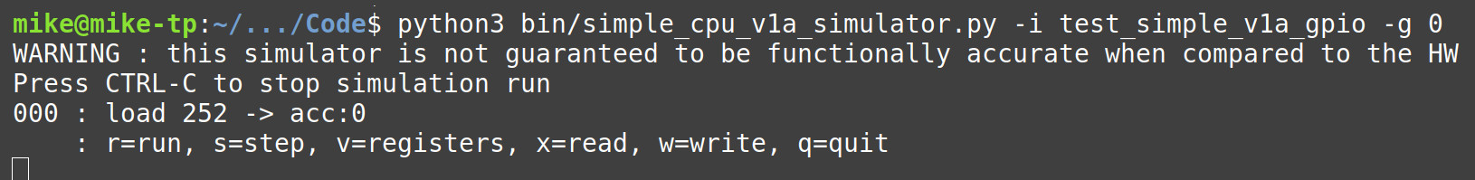
Figure 21 : GPIO enabled, key prompt turned off (top), GPIO disabled, key prompt turned on (bottom)
In the real world the value driven onto the input port would be set by the sensors on the bug trap e.g. switches. In the simulator these have to be set by pressing the i key. This allows the user to enter the values for input port-A and input port-B. Note, only the lower 8bits are used. To view the values on the input and output ports you can use the o key. Pressing this key will display the state of these IO peripheral devices. The values on these GPIO ports can also be read using their memory mapped addresses shown in figure 17.
To test this functionality the test program below was used. Note, the LOAD 0xFC instructions read the input port, the STORE 0xFC instructions write to the output port, they do NOT access RAM :).
########
# DATA #
########

# MEMORY MAP
# ----------
# ADDR   DEC    READ               WRITE
# 0xFF   255    Port B DATA OUT    Port B DATA OUT
# 0xFE   254    Port B DATA IN     Port B DATA OUT
# 0xFD   253    Port A DATA OUT    Port A DATA OUT
# 0xFC   252    Port A DATA IN     Port A DATA OUT
# 0xFB   251    RAM                RAM
# ...    ...    ...                ...
# 0x00   0      RAM                RAM

########
# CODE #
########

start:
  load 0xFC
  and 0x01
  jumpz fire

reset:
  move 0x02
  store 0xFC
  jumpu start

fire:
  move 0x01
  store 0xFC
  jumpu start
In another lab the simpleCPUv1d is used to process an image of Bob the bug, shown in figure 22. This image is a 24 x 24 pixels, 576 pixels in total. This image size was chosen so that you can see Bob, but minimises processing time. Using this image students write assemble language programs to perform simple image processing tasks e.g. extract the blue pixels to generate a blue image of Bob, or mirror this image etc.
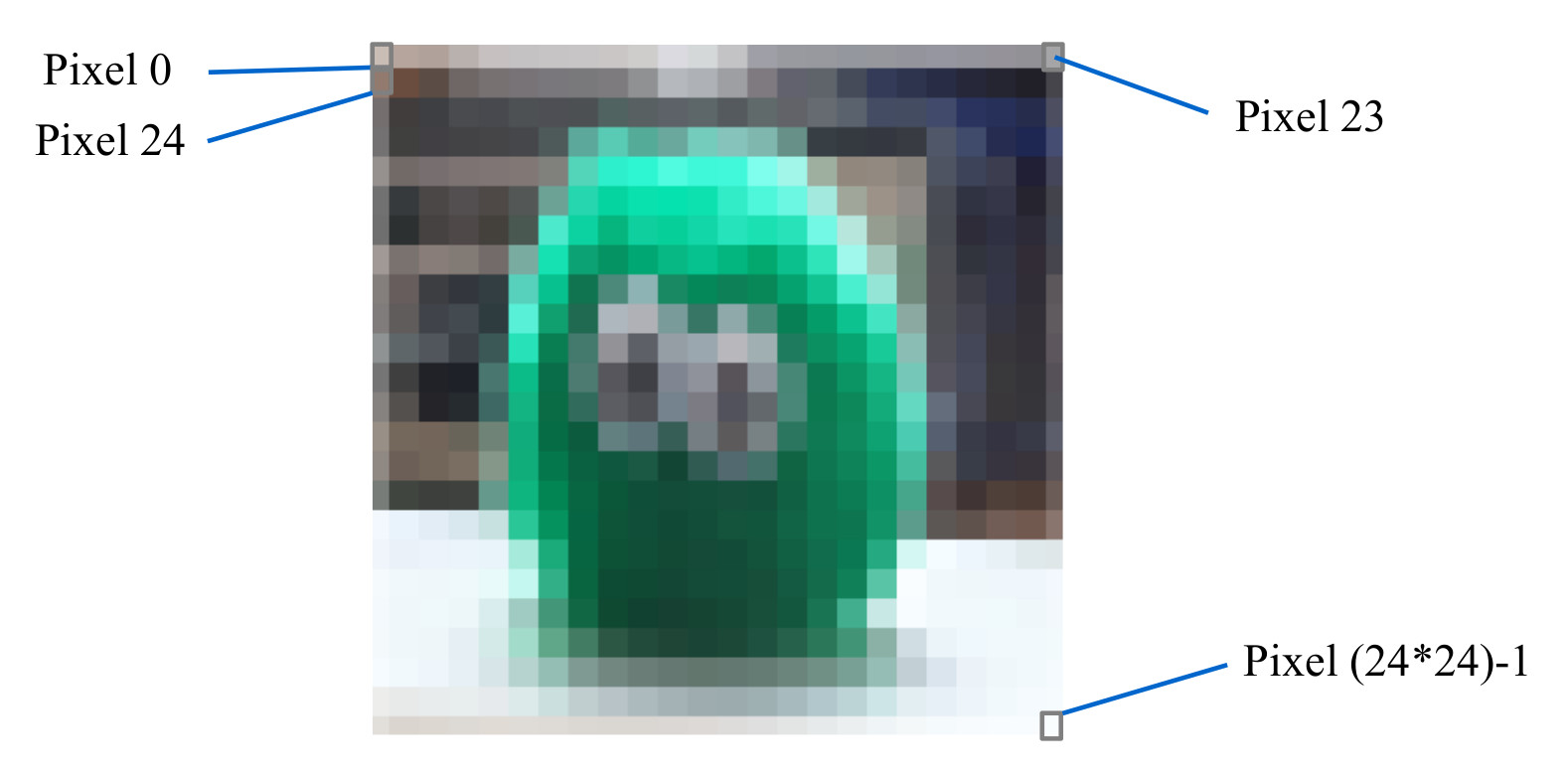
Figure 22 : Bob 24 x 24 image
As the processor's memory is 16bits, 24bit RGB pixel values will not fit into one memory location, therefore, they are stored in the simpleCPU memory using a 5:6:5 RGB packed data type, shown in figure 23. To initialise the simulator's memory PPM images are used owing to their simple format, an example shown in figure 24.
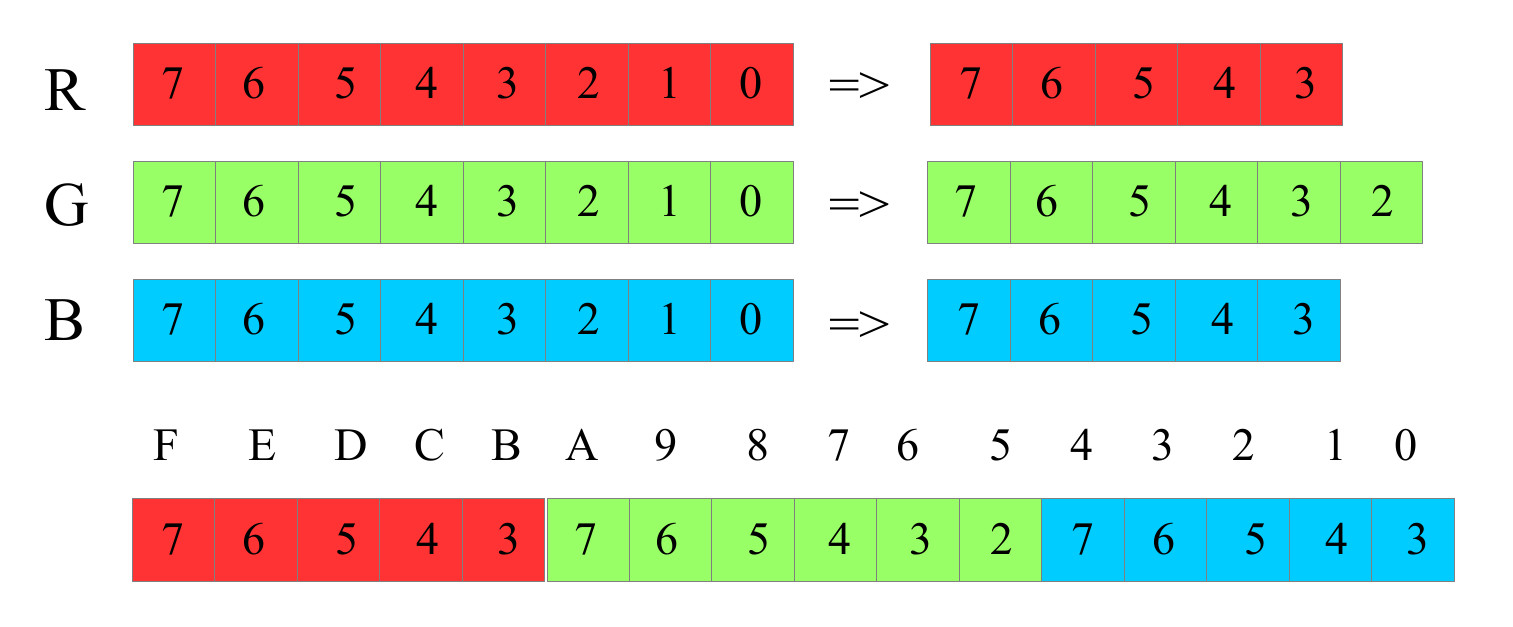
Figure 23 : Packed RGB 5:6:5 format
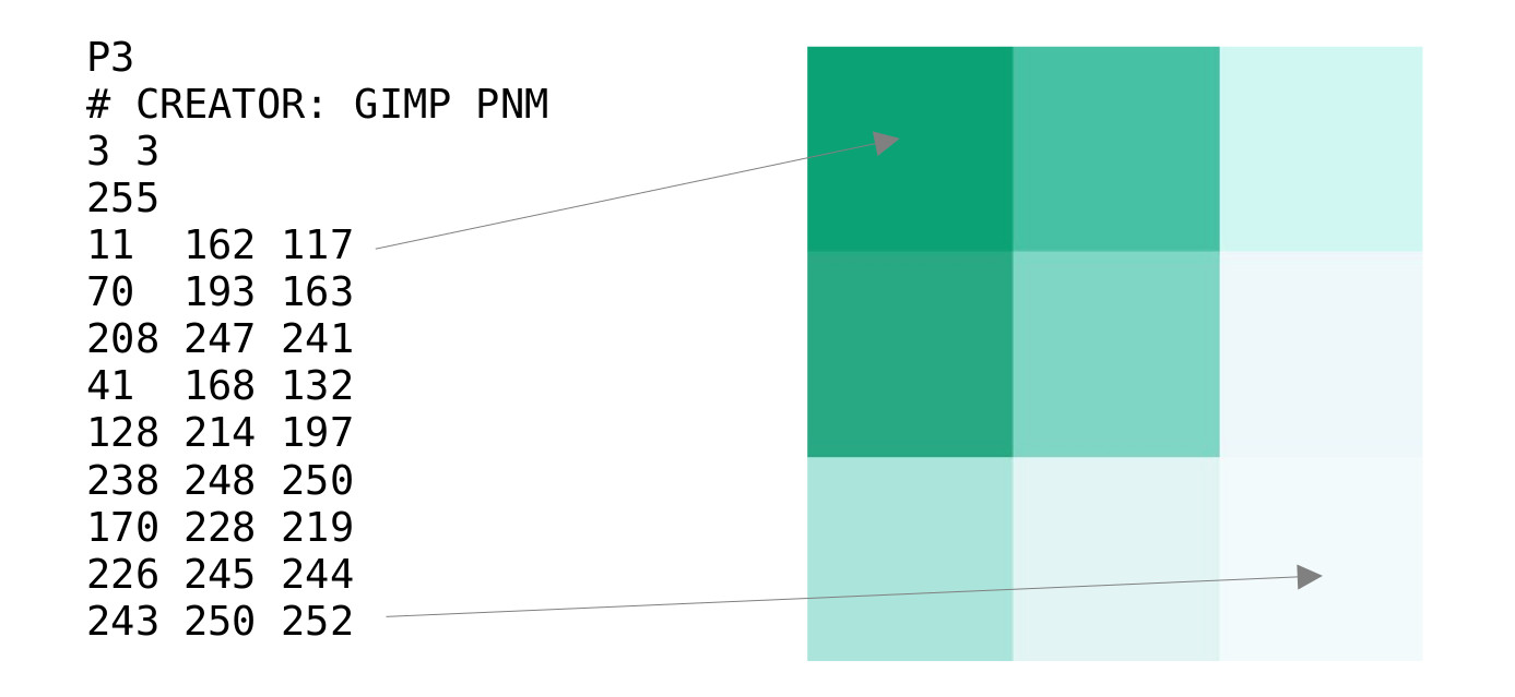
Figure 24 : PPM image format
To enable this image related functionality there are a few more command line options, as shown in figure 25. Note, these are not integrated into the GUI at the moment.
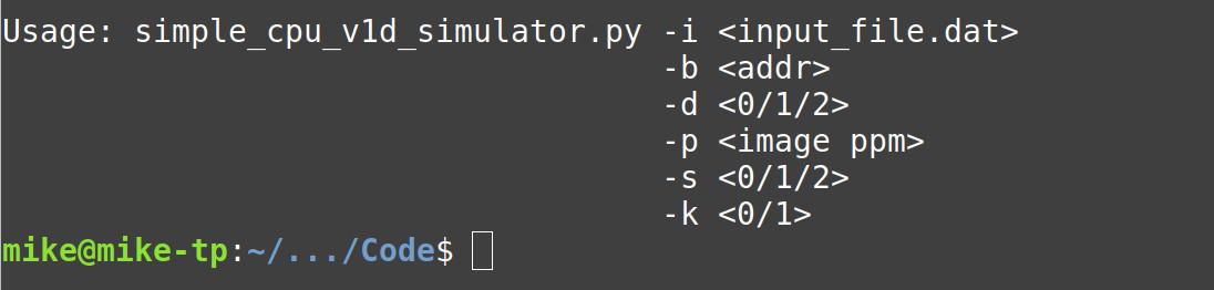
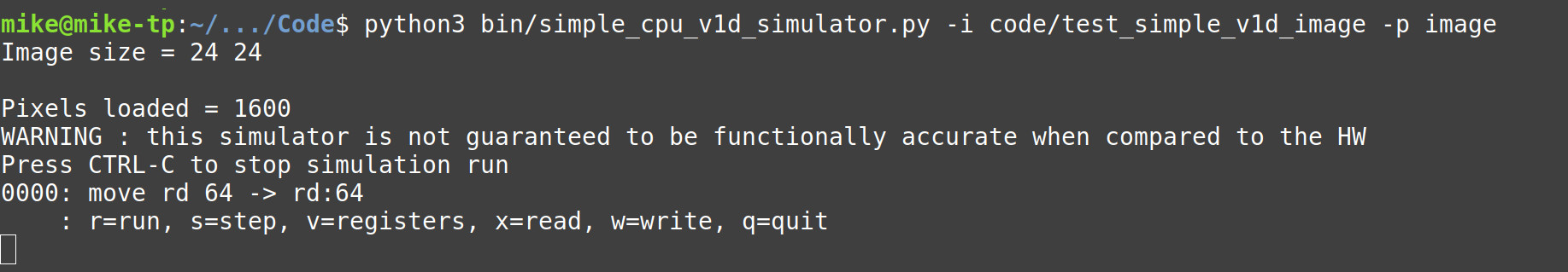
Figure 25 : command line switches
The k and s parameters are as previously defined. The input image filename is specified using the -p parameter e.g. -p image.ppm. If specified this ppm image is loaded into memory. At the movement the base address of where this input image is store is hard coded into the simulator (also the resulting output image's base address) using the variables shown below:
INPUT_IMAGE_BASE_ADDR = 1024
OUTPUT_IMAGE_BASE_ADDR = 1600
If the -p parameter is used the 24bit RGB data in the ppm image file is converted into 5:6:5 RGB values and loaded into memory, starting at the specified base address i.e. 1024. Each memory location stores one pixel. To test this functionality the program below was used. The first program reads each pixel value, zeros the R and G components and stores the B component (unaltered) to a new location i.e. OUTPUT_IMAGE_BASE_ADDR. This process is repeat to create a blue image of Bob. The other program performs a similar function, producing red Bob :).
############
# BLUE BOB #
############

########
# CODE #
########

start:
	move rd 0x40        # set RD to source image
	rol rd              # address
	rol rd
	rol rd
	rol rd
	move rc 0x64        # set RC to output image
	rol rc              # address
	rol rc
	rol rc
	rol rc
	move rb 0x24        # set RB to loop counter
	rol rb
	rol rb
	rol rb
	rol rb

loop:
	load ra (rd)        # read pixel
	and ra 0x1F         # zero all other bits
	store ra (rc)       # save result to memory

	add rd 1            # inc source address pointer
	add rc 1            # inc output address pointer
	sub rb 1            # dec loop counter
	jumpnz loop         # repeat if not zero

	move ra 0xFF        # set output port to all 1s
	store ra 0xFFF      # to trigger image save

stop:
	jump stop           # trap code to finish
###########
# RED BOB #
###########

########
# CODE #
########

start:
	move rd 0x40        # set RD to source image
	rol rd              # address
	rol rd
	rol rd
	rol rd
	move rc 0x64        # set RC to output image
	rol rc              # address
	rol rc
	rol rc
	rol rc
	move rb 0x24        # set RB to loop counter
	rol rb
	rol rb
	rol rb
	rol rb

loop:
	load ra (rd)        # read pixel
	rol ra
	rol ra
	rol ra
	rol ra
	rol ra
	and ra 0x1F         # zero all other bits
	rol ra
	rol ra
	rol ra
	rol ra
	rol ra
	rol ra
	rol ra
	rol ra
	rol ra
	rol ra
	rol ra
	store ra (rc)       # save result to memory

	add rd 1            # inc source address pointer
	add rc 1            # inc output address pointer
	sub rb 1            # dec loop counter
	jumpnz loop         # repeat if not zero

	move ra 0xFF        # set output port to all 1s
	store ra 0xFFF      # to trigger image save

stop:
	jump stop           # trap code to finish
To test these programs the simulator can be run with the -s 2 parameter set, therefore, when the user presses the r key the simulation will run at full speed, automatically halting when it detects the final infinite loop. When the user presses the q key to quit the simulator, it will dump the image stored at the bases address: OUTPUT_IMAGE_BASE_ADDR to the file dump_image.ppm, allowing the user can check if their program has functioned correctly, as show in figure 26.
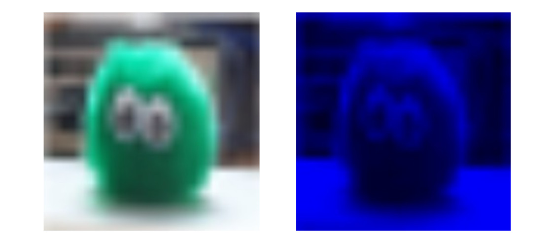
Figure 26 : input image (left), output blue image (right)
Final piece of code needed are a couple of shell script programs to convert the ppm image into the correct format i.e. ppm images can be formatted in different ways. Two common formats are an RGB pixel value per line, or R, G and B values on separate lines. The simulator is expecting data to be formatted with one RGB pixel value per line. So to convert between these formats i use the two shell script programs below. Note, you can find these in the simple_cpu_software.zip download file in the image folder, along with some test images of Bob.
#!/bin/sh

# convert_from_rgb.sh
# -------------------
# converts ppm image file with one RGB pixel value per line to
# one with R, G and B values on separate lines.

if test -z "$1"
then
  echo "Usage: $0 < image.ppm >
  exit 1
fi

input_file="$1"

base_name=$(basename "$1" .ppm)
output_file="${base_name}_single.ppm"

count=0
echo -n > "$output_file"

cat $input_file | while read line
do
  count=$((count + 1))

  case "$count" in
    1|2|3|4)
      echo "$line" >> "$output_file"
      ;;
    *)
      for value in $line
      do
        echo $value >> "$output_file"
      done
      ;;
  esac
done
echo "" >> "$output_file"

echo "Finished! image saved in $output_file"
#!/bin/sh

# convert_to_rgb.sh
# -------------------
# converts ppm image file with with R, G and B values on separate lines
# to one with a single RGB pixel value per line.

if test -z "$1"
then
  echo Usage: $0 < image.ppm >
  exit 1
fi

input_file="$1"

base_name=$(basename "$1" .ppm)
output_file="${base_name}_rgb.ppm"

count=0
length=0
data=""

echo -n > "$output_file"

cat $input_file | while read line
do
  count=$((count + 1))

  case "$count" in
    1|2|3|4)
      echo "$line" >> "$output_file"
      ;;
    *)
      data="$data $line"
      length=$((length + 1))

      if test $length -eq 3
      then
        echo $data >> "$output_file"
        length=0
        data=""
      fi
      ;;
  esac
done
echo "" >> "$output_file"

echo "Finished! image saved in $output_file"
A small update, allowing the simpleCPUv1a simulator to simulate code that uses self modifying code i.e. the two operand STORE instruction. Probably just my coding style, or not knowing better ways of implementing this functionality, but finding python a "joy" when you are trying to get your program to work on different operating systems i.e. Windows and Linux. There are a lot of small differences :(. Soooo, you debug on one OS, test, then when it looks like its all good you try on a different OS, then its stops working. You then discover that the other OS does things just a little differently, just enough to break things :(. This is a particular joy in Windows, as you have different ways in which python can be installed e.g. Anaconda or direct, which results in more code adjustments :(. I think I have found most edge cases, BUT, its starting to get too much fun sooo to simplify my job:
NO SPACES ALLOWED IN FILE NAMES OR DIRECTORY NAMES
On first consideration it may seem that all you need to do is add double quotes, but i found strange things happened with the getopt lib and passing stuff to the command line. So no spaces :). If you spot any other special "features", things that make the software go bang, do left me know. You can download this version here:(version-2).
Some small improvements to both, so grouped these assembler and simulator updates into one section. The assembler had a interesting bug, a lets make a quick improvement bug :), can you spot the issue:
def convertData(data):
  try:
    if '0b' in data:
      return int(data, 2)
    elif '0x' in data:
      return int(data,16)
    else:
      return int(data)
  except:
    print("Error: invalid operand can not convert")
    print(data)
    sys.exit(1)
What i was trying to do was to add support for binary immediate values e.g. 0b10000 = 16 = 0x10. However, we hit an issue with the values 0x0b :). To fix this just needed to swap over the test, as shown below:
def convertData(data):
  try:
    if '0x' in data:
      return int(data,16)
    elif '0b' in data:
      return int(data, 2)
    else:
      return int(data)
  except:
    print("Error: invalid operand can not convert")
    print(data)
    sys.exit(1)
The next improvement linked into the ISim visuliser, a piece of software "i" developed with no AI suuport :), to help students single step through a simpleCPU simulation waveform generated by ISim. This software takes the output of the ISim simulator and rather than viewing this as a waveform diagram it presents this simulation to the user as an instruction trace that they can step through, the user can see the instructions and variables etc. Therefore, this software needs to know the addresses of each variable, sooo, the assembler now outputs two additional files:
LABELS.TXT
This file contains a list of all the labels used in a program and their addresses in memory i.e. labels used to identify instructions (branch targets) and labels to identify data (variables). An example is shown below. For this example program the labels between start and next are instruction labels, whilst the labels data8 and data9 are variable labels.
start 0
loop 196
cmp_eq 206
cmp_neq 209
next 210
data8 263
data9 264
VAR.TXT
This file uses the same syntax, contains a list of all labels used to identify data (variables), sooo, if we consider the previous example this files would contain:
data8 263
data9 264
On reflection could of combined this information into one file, but it was simplier to do this way :).
The instruction set simulator has a number of small modification, these link into thoughts on how to debug assembly language programs (Link). The first improvement was to the x key i.e. how the read memory option works. You can now specify a single address e.g. 10, or a range of addresses e.g. 10-100, or if you don't enter a value the simulator will display all nonzero memory locations. Also added some new command line options, both the simpleCPUv1a and simpleCPUv1d support:
The key improvemnets here are with regards to how test data could be loaded into memory i.e. -p a ppm image, or -l raw data, both of these techniques are discussed in more detail here: (Link).
You can download this version here:(version-3).
Confess its been awhile since i did any GUI design in python. I normally use TkInter and even then it was just your basic boxes and buttons. Sooo, i thought i would give CoPilot a try (other AI tools available) and see what it could code in an afternoon. The answer was depressingly quite a lot :(. My starting point was the block diagram in figure 27. I was looking for a GUI that mirrored this layout i.e. two blocks, processing and variables, with arrows showing the flow of data. Then during the simlation, as the program executed, the processing block i.e. the circle, the instruction's opcode, would be updated with the symbols: + (ADD),| (OR),& (AND),^ (XOR) and ? (JPZ). The current instruction would be displayed in the rectangle "instruction" block, then arrow would be drawn to show where operands were sourced i.e. immediate values from the instruction block and absolute values from variables, and finally an arrow would show where result was stored.
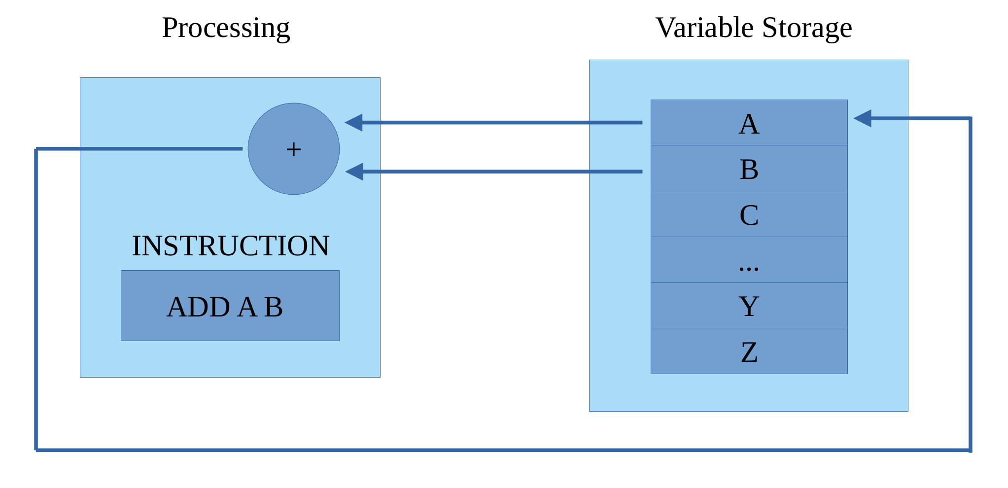
Figure 27 : minimalCPU block diagram
Sooo, in CoPilot is uploaded this image + the existing minimalCPU instruction-set simulator python code + a reasonably descriptive explanation of what i was looking for (less than a page of A4), sorry forgot to save this doc. With this information i got the animated instruction set simulator shown in figure 28.
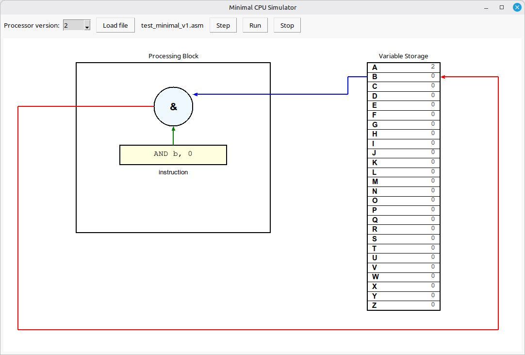
Figure 28 : animated instruction set simulator
This worked pretty much out of the box. The instruction set simulator worked ok, but looking at the code produced that was a cut and paste of my instruction set simulator code. The only part that the AI tools struggled a little with was the arrows, i wanted these to be drawn around the two blocks, with 90 degree bends, rather than straight lines. Also when possible i did not want the blue source operand arrows to cross. Apart from these adjustments it worked first time. I think the trick is to try to be very clear describing what you want, but that is easier said than done. I know this is not a big program, but i was quite impressed what AI tools can do, make you question if it is worth coding small programs. If i had to estimate how long this would have taken me to do, hmmmm, its been a while since i have done any TkInter coding, i have not coded graphics stuff before e.g. arrows, soooo, i would guess a week. Therefore, yes AI did make me more productive, but did i learn anything, no, no i did not :).
If you would like to download this animated instruction-set simulator please use this link:(Link). This zip file contains the python code and some example test programs. To launch the simulator enter the command:
WINDOWS : python animated_minimal_cpu_simulator.py
LINUX   : python3 animated_minimal_cpu_simulator.py
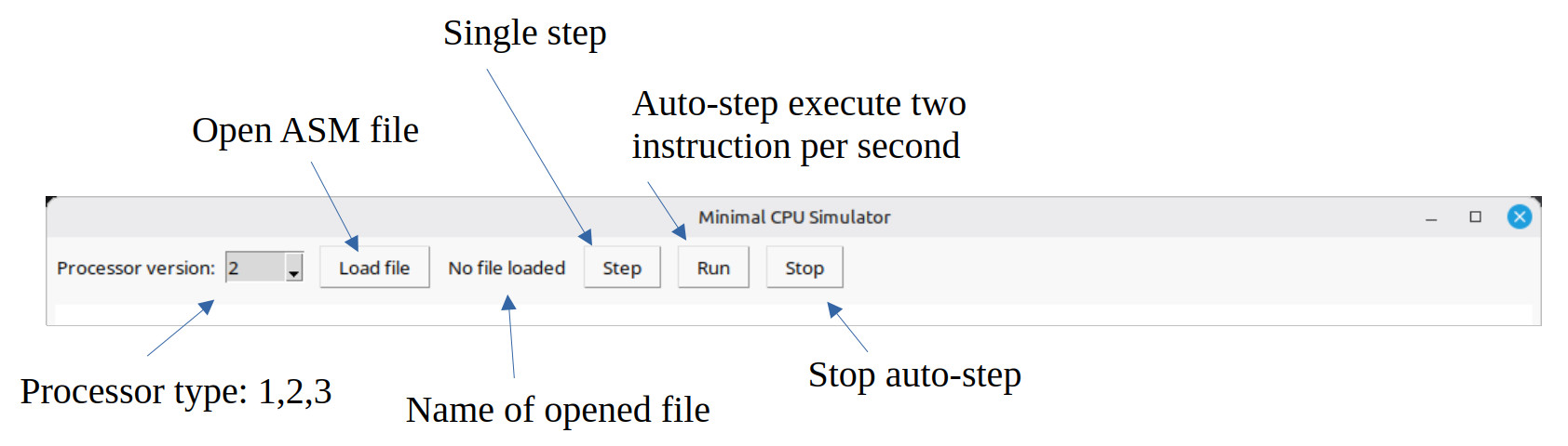
Figure 29 : simulator controls
The simulator controls are shown in figure 29. The user can select the version of the minimalCPU they wish to simulate (1,2 or 3), open the assembly language file they wish to simulate i.e. a plain text file, the assembly language progra. They can then press the Step button to single step through this code, executing one instruction at a time, or the Run button to auto-step through this code, executing an instruction every 400ms, until the program enter an infinite loop where upon it will stop, or until they press the Stop button.
Note, found it interesting that the AI selected 400ms as the auto-step speed, not sure if that links to anything, needs to be slow enough that the user can read the instructions, see the animation, but why 400ms?
WORK IN PROGRESS

This work is licensed under a Creative Commons Attribution-NonCommercial-NoDerivatives 4.0 International License.
Contact email: mike@simplecpudesign.com